Plotting
PegasusTools contains a few features for plotting figures with matplotlib.
Matplotlib Style
A custom Matplotlib style for plotting is defined in PegasusTools and can be used in your scripts. The style sheet is at src/pegasustools/pegasus_style.mplstyle if you wish to see the details.
For a full discussion of how to use style sheets please see the style sheets section of the matplotlib documentation.
[1]:
import matplotlib.pyplot as plt

# To use the PegasusTools style we don't actually need to import PegasusTools, just have
# it installed
plt.style.use("pegasustools.pegasus_style")

# You can also use styles in a context manager
with plt.style.context("pegasustools.pegasus_style"):
    pass

# Styles can be composed together. The rightmost style(s) take priority.
# This works with `plt.style.use` as well
with plt.style.context(["dark_background", "pegasustools.pegasus_style"]):
    pass
Hawley Colormap
The Hawley colormap is not available in any standard packages so it has been included as part of PegasusTools. It will be registered with matplotlib upon importing PegasusTools with the name 'hawley' and can be used as any standard colormap would be; it is also the default colormap in the PegasusTools style sheet.
[2]:
import matplotlib as mpl

import pegasustools as pt  # noqa: F401

mpl.colormaps["hawley"]
[2]:

Example
Below are some examples of the PegasusTools plotting features in action. They are adapted from examples in the matplotlib documentation
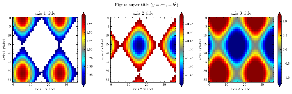
[3]:
import numpy as np

# Note that all plots use the default colormap which is the Hawley colormap in the
# PegasusTools style sheet.

# setup some generic data
N = 37
x, y = np.mgrid[:N, :N]
Z = np.cos(x * 0.2) + np.sin(y * 0.3)

# mask out the negative and positive values, respectively
Zpos = np.ma.masked_less(Z, 0)
Zneg = np.ma.masked_greater(Z, 0)

# Setup figure & suplots
fig, (ax1, ax2, ax3) = plt.subplots(figsize=(13, 3.5), ncols=3)

# plot just the positive data
pos = ax1.imshow(Zpos)

# add the colorbar using the figure's method
fig.colorbar(pos, ax=ax1, extend="both")

# repeat everything above for the negative data
neg = ax2.imshow(Zneg)
fig.colorbar(neg, ax=ax2, extend="both")

# Plot both positive and negative values between +/- 1.2
pos_neg_clipped = ax3.imshow(Z, vmin=-1.2, vmax=1.2)

# Add minorticks on the colorbar to make it easy to read the values off the colorbar.
cbar = fig.colorbar(pos_neg_clipped, ax=ax3, extend="both")
cbar.minorticks_on()

# Text
fig.suptitle("Figure super title ($y= ax_1 + b^2$)")
for i, ax in enumerate((ax1, ax2, ax3)):
    ax.set_xlabel(f"axis {i + 1} xlabel")
    ax.set_ylabel(f"axis {i + 1} ylabel")
    ax.set_title(f"axis {i + 1} title")

plt.show()